index

    Period of a pendulum can be measured by using a light sensor. A laser beam falling on a photo transistor is interrupted periodically by the pendulum. The photo transistor output is fed to one of the digital inputs and the time period is measured by the computer.

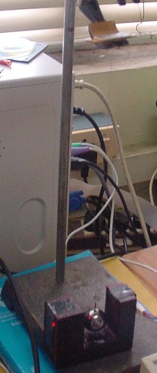
1. Simple pendulum
    The measured values of period 'T' for a pendulum of 29.9 cm length is shown below. Value of 'g' is calculated using the simple pendulum equation. Photograph of the setup.
Period       'g'
1.095241   984.0
1.095222   984.1
1.095241   984.0
1.095229   984.1
1.095230   984.1
1.095223   984.1
1.095191   984.1
1.095165   984.2
1.095196   984.1
1.095205   984.1
1.095179   984.2
1.095178   984.2

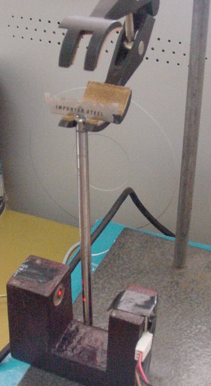
2. Compound pendulum
The values below are for a pendulum made by attaching an iron ball of 1.27 cm radius on one one end of a brass rod of 17.88 cm length and 1.4 mm radius. Photograph
T (usec)     g
0.868908 1001.3
0.868884 1001.4
0.868898 1001.4
0.868877 1001.4
0.868889 1001.4
0.868869 1001.4
0.868886 1001.4
0.868869 1001.4
0.868861 1001.5
0.868867 1001.4
    The value of g is wrong because it is calculated using simple pendulum formula. It can be seen that the period 'T' is measured with an error less than 100 microseconds.

3. Rod Pendulum
The values below are for a 'rod pendulum' of lenght 14.4 cm. The amplitude was decreasing very fast. The calculated value of 'g' changes because of the error due to the assumption sin(theta) = theta changes with amplitude.
0.620988   982.8
0.620955   982.9
0.620907   983.1
0.620854   983.2
0.620805   983.4
0.620767   983.5
0.620714   983.7
0.620660   983.8
0.620614   984.0
0.620568   984.1

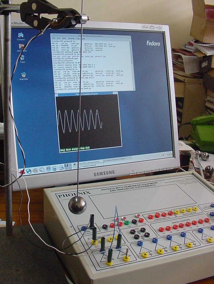
Nature of oscillations
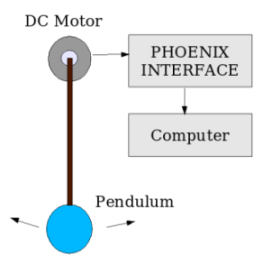
    Simple pendulum can be studied in several different ways depending on the sensor you have got. If you have an angle sensor the displacement of the pendulum can be plotted as a function of time. Since we did not have it we tried to the voltage induced on the terminals of a DC motor when the axis is rotated manually. Some of the motors available in the market has electronic circuits built into it and they are not suitable for our purpose. The experimental setup and output are shown in the figure. The amplitude of the signal is in millivolts only. It is amplified and given to the Digitizer input through the offset amplifier. We got a periodic wave form on the screen when the pendulum connected to the motor axis is set in motion. The period of oscillation can be easily obtained by measuring the distance between the peaks.
setup

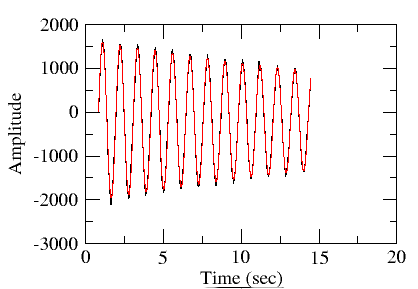
The analysis is done by fitting it with the following equation representing a decaying sinusoidal wave.

The terms theta and C are purely from the experimental setup. If the waveform digitization starts precisely at zero degree theta will vanish and C is the DC offset of the voltage amplifier used. The parameter 'w' gives the angular velocity, and period of oscillation T = 2 * Pi / 5.538 = 1.134 seconds. The length of the pendulum is 32 cm and the value of 'g' calculated from the expression

We used a coil moving inside a magnetic field as the sensor, an old DC motor from a toy car. The voltage produced by a coil rotating inside a magnetic field produces a sine wave. It is a sine wave because the projection of the area of the coil along the magnetic field varies sinusoidally when rotated with a constant speed according to the elementary text books on electricity and magnetism.

Here we are not rotating the coil with a constant speed. The speed changes with angle and we get the peak voltage when the pendulum is vertical, where the angular velocity is maximum. When it moves away from the mean position the voltage should reduce due to two reasons, the change in angular position of the coil (so we thought) and the velocity of the coil . We did not expect a sinusoidal output. In the case of rotation the voltage goes to zero at 90 degree, when the coil is parallel to the field. In case of the pendulum the voltage will go to zero when the pendulum reaches the extreme, may be 20 or 30 degrees from the mean position.

The data shows that the voltage depends only on the velocity. Opening the motor we found that it has multiple poles and there is an axial magnetic field component. The data shows that the voltage induced does not depend on the angular position. Results of fitting with cos² also suggested the same. This needs further exploration by assembling a simple coil in a magnetic field.

Another point is that the sensor does not give the displacement but the time derivative of it. We have used it as if it is the angular displacement and it works because of the sinusoidal nature of the variation. To get angle at any time we need to integrate the values obtained and the constant of integration can be obtained by using a light sensor to mark the time at some known angle. Another method is to attach the pendulum to the axis of a potentiometer and measure the change of resistance. This will directly give the angle information.

The above example illustrates the process of learning physics by explaining experimental data. The insight gained into the subject is beyond what you get by doing the same experiment with a stopwatch. The data analysis techniques required for performing modern experiments also can be taught very effectively.